An oil and gas operator can now hold three methane numbers for one site, and more of the people it answers to compare them. Aircraft and satellites also now detect large releases that an operator may be asked to explain if EPA’s suspended Super-Emitter Program resumes. Over 100 years, a tonne of fossil methane traps about 30 times the heat of a tonne of carbon dioxide [1]. Small errors in a methane inventory therefore carry large climate weight.
EU methane rules as adopted set January 1, 2027 for importers of oil, gas and coal to show EU-equivalent producer-level monitoring, reporting and verification [2]. The duty applies to contracts concluded or renewed on or after August 4, 2024; for earlier contracts, importers must make all reasonable efforts [2]. A non-binding July 2026 Commission recommendation keeps those obligations but asks member states not to apply certain penalties for 2027 to 2029 breaches, fraud excepted [3]. The Commission proposed a one-year delay on October 14, Parliament voted for longer, and a Council mandate backed one year, possibly more; nothing is final.
Emissions intelligence is the work of joining an operator’s reported, modelled and measured methane to the assets behind them. The work explains why the numbers differ and produces one number that holds up. This post covers methane from US onshore oil and gas production for the operators, buyers and compliance teams who have to defend that number. The post explains what each stream measures and at what grain, meaning the unit a number describes, from one valve to a whole basin.
Next come the causes measurement studies have found for the gap between them. The post ends with the reconciliation steps of OGMP 2.0, the Oil and Gas Methane Partnership, and what to look for in software. That section then shows how TetraSoft Atlas, our subscription platform for public well and emissions records, and MAES, our mechanistic emissions model, deliver each stream.
Quick Answer: Emissions intelligence joins three methane data streams to the assets behind them: reported inventories, equipment models and measurements. Alvarez 2018 and Rutherford 2021 found more methane than official inventories. Alvarez traced the gap to abnormal events, and Rutherford to understated tanks and leaks, emission factors and component counts. Comparisons also mislead when a one-day flight is set against an annual total, or when the measurement cannot see small sources. Reconciliation compares like with like, checks the difference against both uncertainties, and adjusts the reported inventory [4].
What Emissions Intelligence Means for Oil and Gas Operators
Emissions intelligence means knowing which methane number applies to which asset, why it differs from the others, and which one to report. Its deliverable can be a site-by-site table. Each row holds a site’s reported number, its modelled range and any measured detections, each with its grain, year and uncertainty. A final column explains the residual, the part of the gap still unexplained after matching.
Each Methane Stream Reports at Its Own Grain
Each stream reports methane at its own grain, from one valve to a whole basin, so two numbers should be compared at a shared grain.
A reported inventory is the operator’s own filing, mostly calculated from equations and emission factors: fixed rates per piece of equipment or unit of activity. EPA says of these factors that “in most cases, these factors are simply averages of all available data of acceptable quality.” [5] The AP-42 Emission Factors by Source Type, and What They Assume post covers what each factor assumes.
A mechanistic model simulates how each piece of equipment behaves, including failures such as a stuck dump valve. The model then sums the results up to the site.
MAES, the Mechanistic Air Emissions Simulator, models “fluid flow through equipment and equipment states.” [6] Measurements come from optical gas imaging, which makes leaking gas visible, and from aircraft, satellites and tower networks. The Leak Detection in Oil and Gas: What Each Method Finds post compares what each can see.
The grain decides what a number can be compared with, and the chart places each source on it.
A component is one fitting, such as a valve, and equipment is one unit, such as a tank or compressor. A site is one well pad or station; a facility is whatever a program counts as one reporting unit, often several sites.
Subpart W of EPA’s Greenhouse Gas Reporting Program treats all of an operator’s onshore production wells in one basin as “one facility.” [7] The 2024 amendments added well and well-pad reporting within that facility from reporting year 2025 [8]. An interim final rule now sets the first reports due March 10, 2027 [9].
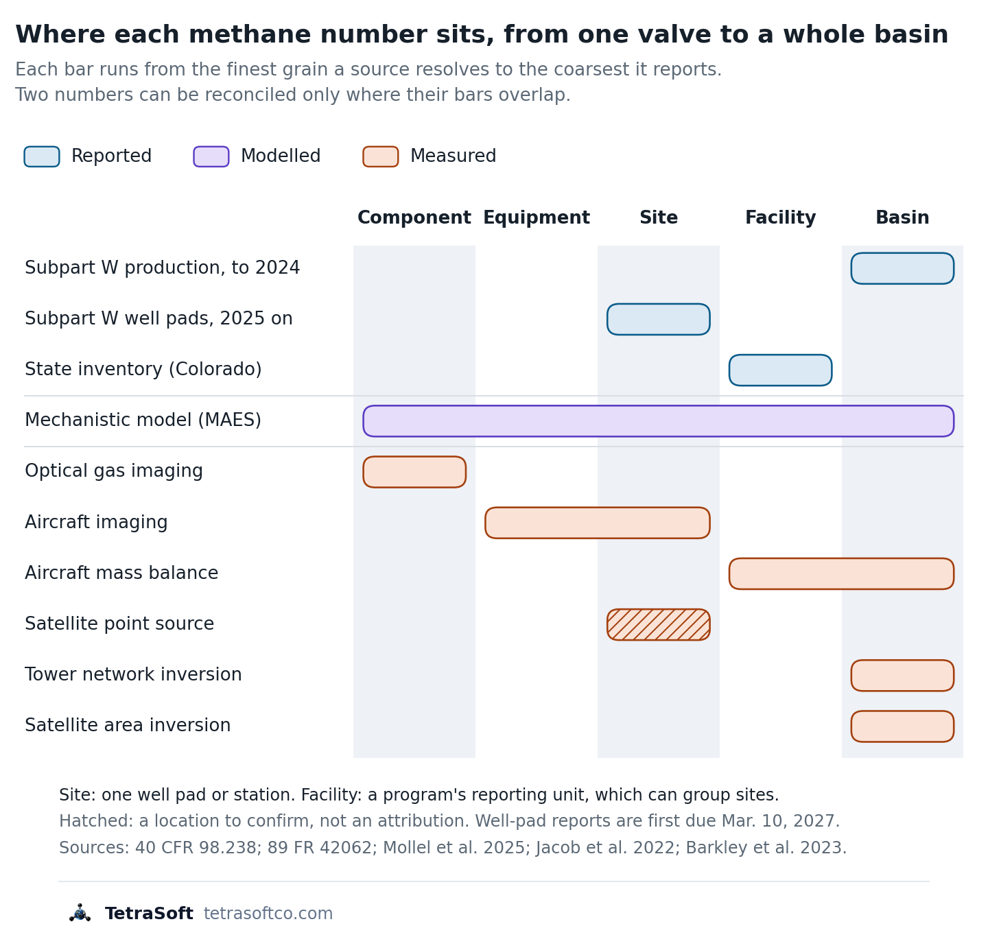
A mechanistic model sums component, equipment and site estimates to facility and basin, so each facility it models can match a measurement’s grain and period.
Point-source satellites are “fine-pixel (< 60 m) instruments designed to quantify individual point sources by imaging of the plumes.” [10]
Such imagers “provide specific facility-level attribution,” so a detection points to a facility [10]. Tower networks estimate basin-scale emissions: one study combined five towers in the Delaware Basin and four in the northeastern Marcellus in an atmospheric inversion [11]. EPA has proposed ending Subpart W reporting for natural gas distribution and suspending the other segments until reporting year 2034; the proposal is not final. The GHGRP Subpart W Reporting in 2026: What Is Still Required post tracks it.
Why Buyers and Regulators Now Ask for It
Three of the programs that bear on the same methane number are described below, and each asks questions a reconciled number helps answer. Two are scheduled from 2027 but now face proposals to delay or repeal them. The EU rule above asks whether imported gas carries monitoring equivalent to the EU’s own, which includes site-level measurement reconciled against source-level estimates [12].
OGMP 2.0, the Oil and Gas Methane Partnership run by the UN Environment Programme, sets five reporting levels [13]. Level 5 adds site-level measurement reconciled against the source-level estimate [13].
OGMP 2.0’s Gold Standard is a status it attributes each year to member companies on a credible path to that top level [14]. To earn it, “a company must achieve Level 4/5 reporting for operated assets within three years and for non-operated assets within five years.” [14] A company that falls off its implementation plan can lose it [14]. The OGMP 2.0 Level 4 and Level 5 Reporting Explained post sets out each level.
In the US, EPA’s Super-Emitter Program wrote third-party measurements into federal rules; it is suspended, and EPA proposed rescinding it on October 29, 2026 [15]. [16] The program lets certified third parties report releases of 100 kilograms an hour or more detected remotely [15]. The operator must then investigate and report the source [15].
The program’s provisions do not apply between July 31, 2025 and January 22, 2027. If the provisions return and survive the proposed rescission, an operator that knows its site-by-site emissions can answer a notice with evidence, not a search.
Why Reported, Modelled and Measured Methane Disagree
Measurement studies have found more methane than US inventories report for over a decade, and they trace the gap to several causes rather than one. Alvarez and colleagues put US oil and gas supply-chain methane at 13 teragrams (million metric tons) a year in 2015, about 60% above EPA’s inventory [17]. Sixty percent is not rounding error.
Causes and Pitfalls the Measurement Studies Identify
The studies trace the gap to abnormal events and missing or understated sources, and one of them also to factors and equipment counts. They also find two ways a comparison can mislead: mismatched time windows and detection limits.
| Cause or pitfall | What the studies found | Study |
|---|---|---|
| A few large, abnormal events | Emission rates are “tail-heavy”, with large emission rates at a small subset of sites; abnormal conditions explain the gap between component-based and site-based estimates | Alvarez et al. 2018; Zavala-Araiza et al. 2017 |
| Sources the inventory omits or understates | Tanks, including failed tank controls, and equipment leaks are the largest contributors to the difference; flares destroy 91.1% of methane rather than the assumed 98% | Rutherford et al. 2021; Plant et al. 2022 |
| Factors and equipment counts | Many inventory data sources date from the 1990s, and equipment counts are estimated from activity such as well numbers; one study found outdated factors unlikely to be the main cause | Rutherford et al. 2021; Alvarez et al. 2018 |
| Different time windows | In one gas basin, manual liquids unloadings peaked in mid-afternoon, when aircraft fly, and comparing methods over very different time scales “can be misleading” | Vaughn et al. 2018 |
| What the measurement can see | A survey’s detection limit leaves smaller emissions out, so a measured total can be a lower bound and understate the gap; point sources emit intermittently | Santos et al. 2025; Jacob et al. 2022 |
Each row is a finding from the named peer-reviewed study; the third row records a disagreement between two of them.
Two of the studies name abnormal operating conditions as the likely cause of the gap. Alvarez and colleagues concluded the inventory falls short “likely because existing inventory methods miss emissions released during abnormal operating conditions.” [17] In a separate Barnett Shale study, site-based estimates exceeded component-based estimates by 52%, a gap the authors attribute to abnormal process conditions [18].
Missing and understated sources come next. In a component-level model, Rutherford and colleagues found “unintentional emissions from liquid storage tanks and other equipment leaks are the largest contributors to divergence.” [19]
Against the national inventory for 2015, tanks alone added about 2.3 teragrams a year [19]. Airborne sampling across the basins behind over 80% of US flaring, combined with unlit-flare surveys, found flares destroyed only 91.1% of methane [20]. That is a fivefold increase in flare emissions above the 98% efficiency inventories assume [20].
The two studies disagree on factors because they tested them differently. Alvarez and colleagues’ EPA-style equipment inventory, rebuilt from recent component measurements, put production within about 10% of EPA’s, though source categories differed significantly [17]. Rutherford and colleagues resampled a more comprehensive component database so that infrequent, large emitters entered the factors, and much of the gap vanished [19].
The measurement side has limits too: a daytime flight can overstate an annual rate, and a detection limit can understate it. Vaughn and colleagues found that “direct comparison of emission estimates from methods covering widely different timescales can be misleading.” [21] The Why Satellites Show About 2x More Methane Than Inventories post explains how satellite inversions work.
What Colorado’s COBE Study Found
Colorado’s COBE study compared aerial surveys with one state’s reported inventory, and its two models gave very different ratios [22]. COBE stands for Colorado Ongoing Basin Emissions [22].
The Colorado health department and Colorado State University’s Methane Emissions Technology Evaluation Center (METEC) ran it on upstream facilities [22]. The study used 2024 data from the state’s Oil and Natural Gas Annual Emission Inventory Reporting program (ONGAEIR) [22]. COBE modelled 9,411 of the 11,681 operating or partially operating upstream facilities with MAES [22].
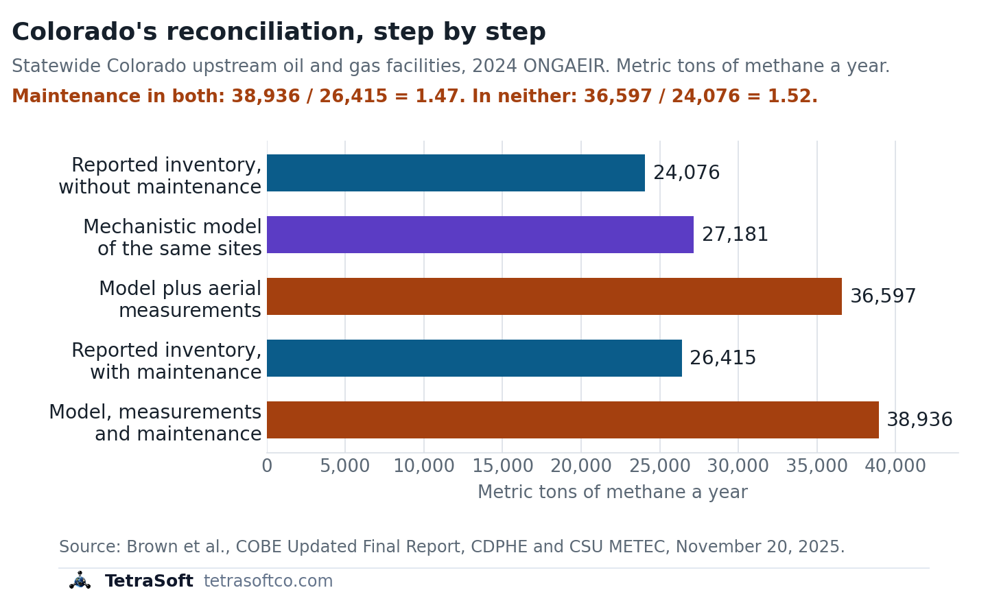
Built from the inventory’s own activity data, the model alone gave 27,181; aerial measurements then added unreported failure emissions.
The MAES model alone came to 27,181 metric tons a year; MAES does not model maintenance, which operators reported at 2,339 [22]. Adding the aerial measurements raised the total to 36,597, and the report attributes the increase to failure events [22].
Maintenance was set aside for the comparison, because aerial surveys cannot reliably quantify such brief events [22]. The operators’ reported maintenance was then added back, for 38,936 metric tons across the 9,411 modelled facilities [22]. A statistical model from the Colorado School of Mines, built on the same flights, gave ratios of 3.30 to 5.09 for the facilities MAES modelled [22]. Across all ONGAEIR facilities, it gave 3.81 to 5.85 [22].
With continuous-monitor data filling in emissions below 5 kilograms an hour, the statistical model put well over half of the modelled facilities’ total there [22]. The report says that model may over- or underestimate those small emissions, while MAES may underestimate them by treating matching detections as already reported [22].
How to Reconcile the Streams, and Where TetraSoft Fits
Reconciliation is the step that turns three numbers into one an operator can report. OGMP 2.0’s uncertainty and reconciliation guidance describes it as “an iterative process of investigation, year over year,” not a one-off comparison [4].
The Reconciliation Steps OGMP 2.0 Describes
Reconciliation compares like with like, checks the difference against both uncertainties, and adjusts the reported inventory [4]. The guidance calls itself “not prescriptive,” so the steps below summarize what it and the EU rule ask for rather than a fixed recipe [4].
- Estimate the uncertainty of both the source-level inventory and the site measurements. The guidance says “reconciliation requires an estimate of uncertainty for both L4 estimates and site level measurements.” [4]
- Measure sites with an independent method and a sampling plan. The guidance warns “a single measurement campaign cannot satisfy both the requirement for source- and site-level measurement,” and that limited-sample estimates “can bias low.” [4]
- Compare like with like. Data “should be reconciled which cover the same sources and which are representative of the same time period,” with source-level estimates summed to each site [4]. [12] COBE’s approach adds corrections for each sensor’s probability of detection and for flights made mostly in daytime [22].
- Test whether the difference is significant. The guidance names Monte Carlo analysis for comparing short measurements with annual estimates, and the EU rule acts on “statistically significant discrepancies.” [4] [12]
- Find the cause and correct the inventory. The operator should “understand the source of discrepancy and transparently report, incorporating any adjustment” to the reported value, then repeat the cycle the next year [4].
Emissions intelligence software can support all five steps, but measurement teams take the site measurements and operators investigate the causes. Look for the grain, year, method and uncertainty on every number, measurements tied to the sites they describe, and a record of each adjustment. The tool below shows the grain of each source before any two are compared.
How TetraSoft Atlas and MAES Deliver Emissions Intelligence
TetraSoft Atlas supplies the reported stream and MAES the modelled one, joined at the grain each question needs. A buyer, an OGMP auditor or an EPA notice asks the same question: why is your number what it is?
TetraSoft Atlas carries public well records for eight states, production records for seven, and emissions records for six. The eight are Colorado, Texas, Wyoming, Pennsylvania, West Virginia, Ohio, Oklahoma and New Mexico; the first six also have emissions records [23]. The eight states produced an estimated 68 percent of US crude oil and 83 percent of US marketed gas in 2025 [24]. We plan to expand Atlas to every US state [25].
In Colorado, Atlas links ONGAEIR facility reports to the wells they list: 38,429 wells whose most recent linked report is for 2025 [26]. Step 1 then starts from the reported number already sitting beside its assets. Operators calculated those figures; the state did not measure them. That is why the reported stream needs a second one to be checked against.
MAES, the Mechanistic Air Emissions Simulator, supplies the modelled stream from component to basin for each facility it has the inputs to model. MAES uses Monte Carlo methods to capture the variability in facility operations, and its runs give a probability distribution of emissions for each facility [22]. The range is built up from each piece of equipment and the leak-prone components on it.
Set against each technology’s probability of detection, that range shows whether a technology “can actually see what is at your site” before a campaign. With measurement data added, the same model becomes a measurement-informed inventory; with reported maintenance added too, COBE’s was 1.47 times ONGAEIR’s 26,415 metric tons [22]. Both totals in that ratio include the operators’ reported 2,339 metric tons of maintenance, plus unmodelled dehydrator, internal combustion engine and pneumatic pump emissions [22]. Without maintenance on either side, the report puts the MAES measurement-informed total of 36,597 metric tons 52% above the adjusted reported inventory [22].
In the Denver-Julesburg Basin, that method estimated an additional 16.4% of total emissions from abnormal events, using operator inventories and Carbon Mapper aerial measurements [27]. This post’s author, Arthur Santos, first-authored that study, co-authored the MAES model study and the COBE report, and co-founded TetraSoft. MAES was developed through research that includes the EEMDL initiative of CSU and UT Austin, and TetraSoft offers it through a special license with CSU [28].
Start with the reported stream: see Colorado ONGAEIR facilities next to their wells in TetraSoft Atlas, free for seven days with no credit card. No measurements yet? “No field measurement hardware is required for a baseline simulation” in MAES.
Frequently Asked Questions
What does OGMP stand for?
OGMP stands for the Oil and Gas Methane Partnership [14]. OGMP 2.0 is the UN Environment Programme’s reporting framework for oil and gas methane [14]. OGMP 2.0 has five reporting levels, and Level 5 adds site-level measurement reconciled against the source-level inventory [13].
Is methane worse than CO2?
Per tonne, yes: over 20 years a tonne of fossil methane traps about 83 times the heat of a tonne of carbon dioxide [1].
The gap narrows with time because methane lasts about 12 years in the atmosphere [1]. Carbon dioxide’s added concentration lasts thousands of years [29].
How do satellites detect methane?
Satellites measure how much sunlight methane absorbs in the air column beneath them [10]. Area-flux instruments with pixels of 0.1 to 10 kilometres estimate regional totals, while point-source imagers with pixels under 60 metres map individual plumes [10].
Have measurement campaign data, or want a baseline first? Contact us and we will build your Measurement-Informed Inventory with MAES.
This post is for informational purposes only and does not constitute legal or compliance advice. Consult qualified legal counsel or a compliance professional for guidance specific to your operations and jurisdiction.
References
- IPCC AR6 WG1, Chapter 7, Table 7.15
- Regulation (EU) 2024/1787, Article 28
- Commission Recommendation (EU) 2026/1835, July 20, 2026, on penalties for importers’ methane obligations, Official Journal of the European Union, July 24, 2026
- OGMP 2.0 Reconciliation and Uncertainty Guidance, Steering Group approved, 2022, ogmpartnership.org, accessed September 30, 2026
- EPA, Basic Information of Air Emissions Factors and Quantification, accessed September 22, 2026
- Mollel et al., ACS ES&T Air, 2025, 2, 723-735, DOI 10.1021/acsestair.4c00168
- 40 CFR 98.238, Definitions, Subpart W (Petroleum and Natural Gas Systems)
- 89 FR 42062, Greenhouse Gas Reporting Rule: Revisions and Confidentiality Determinations for Petroleum and Natural Gas Systems, May 14, 2024
- 91 FR 65112, Extending the Reporting Deadline Under the Greenhouse Gas Reporting Rule for Reporting Year 2025 to March 10, 2027, interim final rule, October 14, 2026
- Jacob et al., Atmospheric Chemistry and Physics, 2022, 22, 9617-9646, DOI 10.5194/acp-22-9617-2022
- Barkley et al., Atmospheric Chemistry and Physics, 2023, 23, 6127-6144, DOI 10.5194/acp-23-6127-2023
- Regulation (EU) 2024/1787, Article 12
- UNEP OGMP 2.0 Module 2, The OGMP 2.0 reporting levels, August 2025
- OGMP 2.0 Frequently Asked Questions, ogmpartnership.org, accessed September 29, 2026
- 40 CFR 60.5371b, Super-emitter response program
- 91 FR 68234, Additional Reconsideration of Standards of Performance for New, Reconstructed, and Modified Sources and Emissions Guidelines for Existing Sources: Oil and Natural Gas Sector Climate Review, proposed rule, October 29, 2026
- Alvarez et al., Science, 2018, 361(6398), 186-188, DOI 10.1126/science.aar7204
- Zavala-Araiza et al., Nature Communications, 2017, 8, 14012, DOI 10.1038/ncomms14012
- Rutherford et al., Nature Communications, 2021, 12, 4715, DOI 10.1038/s41467-021-25017-4
- Plant et al., Science, 2022, 377, 1566-1571, DOI 10.1126/science.abq0385
- Vaughn et al., PNAS, 2018, 115, 11712-11717, DOI 10.1073/pnas.1805687115
- Brown et al., Colorado Ongoing Basin Emissions (COBE) Updated Final Report, November 20, 2025
- TetraSoft Atlas state coverage registry, read September 30, 2026
- U.S. Energy Information Administration, crude oil and natural gas marketed production by state, annual 2025, accessed September 23, 2026
- TetraSoft Atlas landing page, tetrasoftco.com/atlas-landing.html, accessed September 30, 2026
- TetraSoft Atlas canonical store, counted September 30, 2026
- Santos et al., ACS ES&T Air, 2025, 2, 1598-1611, DOI 10.1021/acsestair.5c00089
- TetraSoft, MAES Platform product page, accessed September 23, 2026
- EPA, Understanding Global Warming Potentials, accessed September 29, 2026
Interactive tool
Can this emissions number be pinned to a well?
Pick a methane data source. See the grain it reports at, whether its number describes one well site, and the source at the same grain to reconcile it against.
Pinned to a single well site?
No
It describes a whole basin; pinning it to a well needs an allocation method.
- Basin
- Facility
- Site
- Equipment
- Component
- Stream
- Reported
- Grains it covers
- Basin grain
- Reconcile it against
- A satellite or tower inversion for the same basin and year
- What it misses
- Which well or site emitted, and failures an average factor smooths away.
Grains as set out in this post: 40 CFR 98.238, 89 FR 42062, Mollel et al. 2025, Jacob et al. 2022 and Barkley et al. 2023, read September 29, 2026. Methane from US onshore production. The EPA National Emissions Inventory is not listed because its oil and gas grain was not verified for this post.
Comments
0Share your thoughts. All comments are moderated before appearing.
No comments yet. Be the first to share your thoughts!