Leak Detection in Oil and Gas: What Each Method Finds

Methane leak detection covers several methods that answer different questions, and the differences between them are larger than the marketing suggests. Optical gas imaging, handheld laser instruments, fixed continuous monitors and aerial surveys each detect a different minimum emission rate under different conditions. Controlled release is the most direct test of what a method finds, because the emitted rate is known on every trial. That includes the trials where the surveyor found nothing, which is what fixes the miss rate. Other designs count misses too, in aggregate rather than trial by trial. An aerial inventory scales its measured rate distribution by a detection curve to estimate what sat below the limit [1]. A measured regional total can also be set against the government inventory. Nearly one million aerial site measurements across six US regions came out near three times the national estimate [2]. Quantification has fallen short for continuous monitors [3]. One 2024 single-blind test found the five systems that reported a rate underestimated by about 74 per cent on average [3]. They also show that who runs the survey changes the result [4].

Quick Answer: Controlled-release testing of optical gas imaging measured detection well below what earlier camera studies implied [4]. The leak size needed for a 90 per cent probability of detection was an order of magnitude larger than earlier camera-focused studies [4]. Surveyors who had covered more than 551 sites detected 1.7 times more leaks than less experienced surveyors [4]. A quarterly survey observes under a fifth of one per cent of the year.

What Controlled Releases Show Each Method Detects

A detection method is characterised by the smallest emission it reliably finds, not the smallest it can ever find. Probability of detection rises with emission rate, so a method is described by the rate at which it finds a set share of releases. Instrument specifications describe the sensor and controlled releases describe the survey.

Controlled release is the method behind both studies below. Gas is released at a known rate from a known component, and the surveyor works the site normally.

Method	What it senses	What a controlled release measures
Optical gas imaging	Infrared absorption, viewed as a plume	Whether a surveyor finds a release of known size
Handheld laser	Path-integrated methane concentration	The rate below which detection becomes unreliable
Fixed continuous monitors	Concentration at a point, over time	Detection and localisation across changing wind
Aerial survey, source level	A plume resolved and tied to one emitter, by laser or by sunlight absorption	The rate found from altitude in one overpass
Aerial survey, mass balance	Downwind flux for a whole site or basin, with no attribution	The total the flight recovers against a known release
Satellite survey	Column methane averaged over a pixel, revisited on an orbit	The rate large enough to clear a coarse pixel

Aerial is not one method. A source-level survey resolves individual emitters and attributes each one to a piece of equipment [1]. It does that either by active laser, as in Bridger’s gas mapping LiDAR [1]. Or by reading sunlight absorption with a passive spectrometer, as in Insight M’s LeakSurveyor [5]. A mass-balance flight instead measures the flux leaving a whole site or basin and attributes none of it. The two are not substitutes: one tells you which unit to fix, the other tells you the total you are missing.

Each row answers a different question, so the methods are not substitutes for one another.

Optical Gas Imaging Depends on the Surveyor, Not Only the Camera

The largest published test of optical gas imaging measured people rather than cameras [4]. Professional surveyors from 16 oil and gas companies and 8 regulatory agencies completed 488 tests over ten months [4]. Surveyors used their own cameras and their own protocols at an outdoor facility built to resemble upstream operations [4].

Two findings from that study are worth carrying. Detection rates were significantly lower than in earlier studies that focused on camera performance [4]. The leak size needed for a 90 per cent probability of detection was an order of magnitude larger than those earlier studies reported [4].

Experience then moved the result again [4]. Surveyors from operators and contractors who had surveyed more than 551 sites detected 1.7 times more leaks [4]. The reported confidence interval on that ratio runs from 1.5 to 1.8 [4]. Experienced surveyors adjusted their speed and examined components from several viewpoints [4].

A camera specification cannot express any of that. Two operators running the same camera model to the same regulation can return materially different detection rates.

Handheld Lasers Were Tested the Same Way

Handheld laser instruments went through a controlled-release assessment at METEC during 2025 [6]. The test used 279 controlled natural gas releases across 20 days [6]. Thirty surveyors from ten operators took part, using four commercially available devices [6].

All four devices performed with detection limits below 0.6 kilograms per hour in the 2025 testing [6]. That study is still underway and its authors describe the results as preliminary [6]. That figure is the useful one to carry, because it is a rate rather than a concentration.

The contrast with concentration-based screening matters here. A concentration threshold tells a surveyor that gas is present at a component. A rate-based detection limit can be set against how much a site is expected to emit.

The controlled-release literature is larger than the two studies above. The table lists controlled-release tests by method class, most of them single-blind. Rates and results are quoted as each study states them.

Study	What was tested	Release rates	Headline result
Ravikumar et al. 2018	Infrared camera, controlled distance	g/h methane	50 per cent detection near 20 g/h at 6 metres
Zimmerle et al. 2020	Optical gas imaging, 488 surveyor tests	methane, scfh	90 per cent detection near 7 scfh for the most experienced surveyors, an order of magnitude above camera studies
Sherwin et al. 2021	Airplane hyperspectral imaging	18 to 1,025 kg/h methane	182 of 200 releases found, no false positives in 21 blanks
Bell et al. 2022	Aircraft LiDAR, 650 passes	0.08 to 1,428 kg/h methane	87 per cent of quantifications within a factor of two
Conrad, Tyner and Johnson 2023	Bridger LiDAR, 495 releases, plus published data for two platforms	0.4 to 66 kg/h methane, Bridger	Detection curves fitted to rate, wind and altitude
Bell et al. 2023	Eleven continuous monitors	0.4 to 6,400 g/h methane	90 per cent detection 3 to 30 kg/h for 8 of 11, upper end extrapolated, false positives 0 to 79 per cent
Sherwin et al. 2024	Nine satellite systems	0.03 to 1.48 t/h methane	55 per cent of estimates within 50 per cent of the metered value, no false positives in 11 blanks
Chen et al. 2024	Eight continuous monitors, high volume	0.037 to about 2,830 kg/h methane	All five systems that reported quantification underestimated, by about 74 per cent on average
Day, Levin and Zimmerle 2025	Four handheld lasers, 279 releases	kg/h methane	All four below 0.6 kg/h at 90 per cent detection, preliminary
Cheptonui et al. 2025	Thirteen continuous monitors	0.08 to 6.75 kg/h methane	90 per cent detection 0.5 to 6.7 kg/h for six of thirteen

Controlled-release studies, by the method class each one tested.

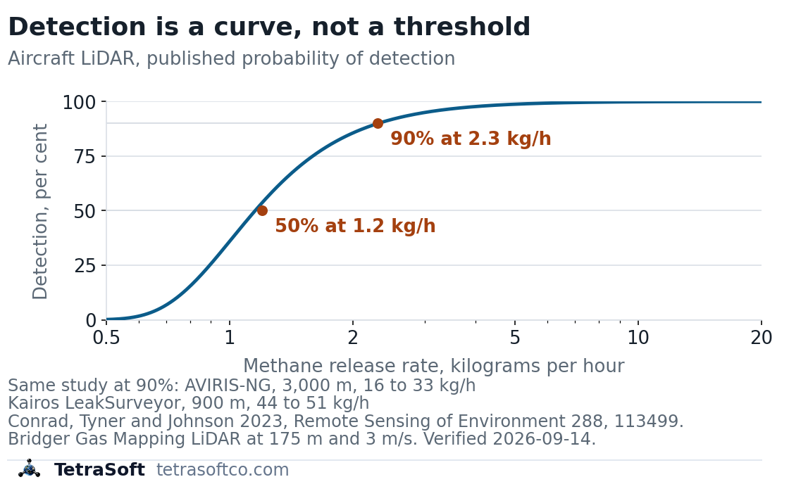
Published probability of detection for Bridger Gas Mapping LiDAR at 175 metres and 3 metres per second, from the fitted equation in Conrad, Tyner and Johnson 2023. The curve moves with altitude and wind, which is why a detection limit quoted without both is incomplete.

Two conventions are in use and they do not agree. Some studies report a wind-normalised limit, in kilograms per hour per metre per second [7]. Others fit detection as a function of rate, wind and altitude together [1]. A detection limit quoted without a wind speed and an altitude is therefore incomplete.

Different Methods Find Different Emissions

Two methods run over the same sites do not return the same picture [8]. Wilde et al. (2025) compared three years of regulated LDAR survey data against independent aerial surveys of the same well sites in British Columbia [8]. At 326 sites covered by both, the aerial surveys detected twelve times more methane than the ground LDAR program [8]. That figure counts everything the aircraft saw, including combustion and deliberate venting a component survey is not looking for [8]. Excluding those leaves a fourfold difference, which is the like-for-like number [8].

The same study measures what the ground programme does achieve [8]. At fully compliant sites, three comprehensive surveys a year reduced detected emission sources by 51 per cent [8]. Counting the sites that fell short of the survey schedule, the programme delivered a 40 per cent reduction overall [8].

The inversion underneath that number is the useful part [8]. Ground LDAR found 2.7 times more individual sources than the aerial survey did [8]. Those sources emitted at 33 times lower rates each [8].

	Sources per site	Mean rate per source
Ground LDAR survey	3.9	0.34 kg/hr
Aerial survey	1.4	11 kg/hr

Ground surveys found many small sources and the aerial survey found few large ones, over the same sites. [8]

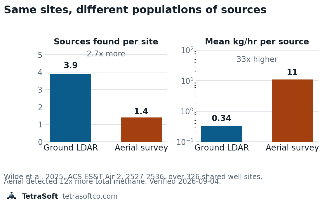
The method decides which population of sources you see, not how thoroughly you looked.

Neither result makes the other wrong. Eighty-two per cent of the sources ground LDAR found were connectors, valves or other small components [8]. Connectors and valves are exactly what a walking survey is built to inspect.

A properly run survey programme does reduce emissions, by the margins given above [8]. What it cannot do is see the rest of the year.

What a Periodic Survey Observes of the Year

Detection limit answers what a survey can see, and it leaves open when the survey is looking. A periodic survey observes a site for a few hours and then leaves. An emissions inventory covers 8,760 hours.

The arithmetic is unflattering and rarely stated. Four quarterly surveys of four hours each observe 16 hours of a year. The four hour figure is an assumption rather than a measured average. That is under a fifth of one per cent of the year.

Raising survey frequency moves that number less than intuition suggests. Moving from annual to monthly surveys multiplies observed time by twelve. It still leaves observed time near half a per cent of the year.

Why the Gap Matters When Emissions Are Episodic

Sampling gaps matter in proportion to how uneven the emissions are. Zavala-Araiza et al. (2017) found that super-emitters in natural gas infrastructure are caused by abnormal process conditions [9]. The finding was published in Nature Communications [9].

Abnormal conditions are by definition not the state a site is usually in. A survey that observes a fifth of one per cent of the year is unlikely to be present during one. Satellite and aerial surveys extend coverage across area rather than across time, and their trade-offs are covered in Why Satellites Show About 2x More Methane Than Inventories.

Continuous monitoring changes the observation problem rather than the detection problem. A fixed monitor sees the whole year at whatever rate it can resolve.

Where Detection Ends and Inventory Begins

Detection and inventory are different products of different processes. A leak detection and repair program finds and fixes individual leaks. An inventory states how much a site emitted over a reporting period.

Survey frequency is set in the federal standards, whose own status is uncertain as of September 2026. The federal rule is not the whole of the requirement. Colorado’s Regulation 7 sets its own tiered inspection schedule for well production facilities, running from annual to monthly by facility category [10]. An operator in a state with its own programme follows whichever schedule is stricter, and What Is Subpart W Suspension? State Rules Still Apply covers why the state layer outlives federal change. Their scope is covered in EPA OOOOb Explained: Who It Covers and What It Requires. Those standards set how often a site is visited rather than how much it emitted between visits.

What a Detection Program Cannot Tell You

A repair log is not an emissions total, and treating it as one hides the gap. Counting leaks found says nothing about the mass released before they were found. It also says nothing about emissions below the detection limit.

Reporting frameworks separate the two deliberately. The distinction between survey-based and quantified reporting is covered in OGMP 2.0 Level 4 and Level 5 Reporting Explained.

Where a Measurement-Informed Inventory Fits

TetraSoft does not run leak detection surveys, and MAES does not detect leaks. It cannot tell an operator that a specific valve is leaking now. That boundary is worth stating before any claim about what it does.

MAES is a mechanistic emissions model developed at CSU and UT Austin, which TetraSoft uses through a partnership with CSU [11]. A survey returns a rate at one moment, and an inventory needs a mass across a year. Bridging the two takes the one quantity a snapshot cannot supply, which is how often a source sits in its failed state [12]. The model produces the normal-operation distribution each detection is judged against, then turns an observed failure frequency into an annual figure [12].

That method has been run on real sites [12]. Across 19 partner midstream facilities in the Appalachian Basin, measured abnormal-process emissions were added to a calibrated baseline [12]. That put the annual methane estimate 58.9 per cent above what those operators reported for normal operation [12]. Against their total reported inventory, fugitives included, the increase was 40.0 per cent [12]. The revision sat in produced water tanks and compressor crankcases, neither of which the 2022 reporting rules required [12]. It also sat in compressor seals found to have failed during the field surveys [12].

Three cautions belong with that number. The authors report it as the contribution of previously unreported sources, not as an independent discrepancy between two estimates [12]. Nineteen facilities from two operators are not a representative sample [12]. The model does not implement emergency shutdowns or maintenance blowdowns, which makes both figures a lower bound [12]. The corresponding author of that study is employed by TetraSoft [12].

An operator choosing between a quarterly program and a monthly one is choosing between 0.18 per cent of the year and 0.55 per cent. Neither figure covers the hours when nobody is on site, which is the gap the MAES platform is built to estimate. The same method was applied earlier in the Denver-Julesburg Basin, where it is documented in full [13].

Frequently Asked Questions

Why do controlled-release results differ from instrument specifications?

Because they measure different things. A specification is established on the instrument under favourable conditions. A blind controlled release measures a surveyor finding an unknown release on a working site [4].

Does more frequent surveying substitute for continuous monitoring?

Not on observed time, whatever it does for repair speed. Weekly four-hour surveys observe about 2.4 per cent of a year. Continuous monitoring observes all of it, subject to its own minimum detectable rate.

What should an operator ask a survey contractor for?

Ask how many sites the assigned surveyors have personally covered. The experience threshold that separated the two groups in the published test was 551 sites [4]. A bid priced per site says nothing about who will be holding the camera.

Can a leak detection program produce an emissions inventory?

Not on its own, because it records findings rather than mass over time. Emissions below the detection limit leave no record at all. Quantification requires either measurement of the source or a model of the site.

Which method should an operator choose?

That depends on which question is being asked, and most programs end up using more than one. Choose on the minimum detectable rate you need and the share of the year you need observed. Treat a vendor specification as a starting point and ask for controlled-release results.

What is LDAR, and what does it cover?

LDAR stands for leak detection and repair, a program of scheduled surveys rather than a single instrument. It covers components that leak when they wear or seat badly, such as valves, connectors, flanges, seals and thief hatches. The survey method is a separate choice from the program itself.

What is the difference between LDAR and optical gas imaging?

LDAR is the program and optical gas imaging is one way to carry it out. A handheld laser, a fixed monitor or an aerial survey can serve the same program. The program sets how often you look, and the method sets what you find when you do.

Can a survey tell whether an emission is persistent or intermittent?

Not from one visit. A detection records that gas was escaping while the surveyor was present, not how long it had been. This matters because the largest emissions tend to come from abnormal conditions rather than steady operation [9]. Repeat visits or a continuous monitor are what separate a persistent source from an excursion.

Interested in building a Measurement-Informed Inventory for your operations? Contact us to learn about our MAES-based estimation services.

---

References

1. Zimmerle et al., 2020, Environmental Science and Technology, 54, 11506-11514, DOI 10.1021/acs.est.0c01285. “Detection Limits of Optical Gas Imaging for Natural Gas Leak Detection in Realistic Controlled Conditions.” https://doi.org/10.1021/acs.est.0c01285
2. Day, Levin and Zimmerle, 2025, CSU Energy Institute METEC, handheld laser controlled-release assessment, preliminary. “Handheld Laser-Based Methane Leak Detection Device Performance During Controlled Natural Gas Releases.” Research poster summary; the authors state results are preliminary and the study is ongoing. https://metec.colostate.edu/handheld-laser/
3. Wilde et al., 2025, ACS ES&T Air, 2, 2527-2536, DOI 10.1021/acsestair.5c00195. “The Efficacy of Methane Leak Detection and Repair (LDAR) Programs in Practice.” https://doi.org/10.1021/acsestair.5c00195
4. Zavala-Araiza et al., Nature Communications, 8, 14012, 2017. “Super-emitters in natural gas infrastructure are caused by abnormal process conditions.” https://doi.org/10.1038/ncomms14012
5. Mollel et al., 2025, ACS ES&T Air, 2, 723-735, DOI 10.1021/acsestair.4c00168. “Using Prototypical Oil and Gas Sites to Model Methane Emissions in Colorado’s Denver-Julesburg Basin Using a Mechanistic Emission Estimation Tool.” https://doi.org/10.1021/acsestair.4c00168
6. Santos et al., 2025, ACS ES&T Air, 2, 1598-1611, DOI 10.1021/acsestair.5c00089. “Using Measurement-Informed Inventory to Assess Emissions in the Denver-Julesburg Basin.” https://doi.org/10.1021/acsestair.5c00089
7. Santos et al., 2026, Gases, 6, 44, DOI 10.3390/gases6030044. “Beyond Snapshots: Building Methane Measurement-Informed Inventories for Midstream Oil and Gas Sites in the Appalachian Basin.” https://doi.org/10.3390/gases6030044
8. Chen et al., 2024, ACS ES&T Air, 1, 871-884, DOI 10.1021/acsestair.4c00015. “Comparing Continuous Methane Monitoring Technologies for High-Volume Emissions: A Single-Blind Controlled Release Study.” https://doi.org/10.1021/acsestair.4c00015
9. Ravikumar et al., 2018, Environmental Science and Technology, 52, 2368-2374, DOI 10.1021/acs.est.7b04945. https://doi.org/10.1021/acs.est.7b04945
10. Sherwin et al., 2021, Elementa, 9, 00063, DOI 10.1525/elementa.2021.00063. https://doi.org/10.1525/elementa.2021.00063
11. Bell et al., 2022, Elementa, 10, 00080, DOI 10.1525/elementa.2022.00080. https://doi.org/10.1525/elementa.2022.00080
12. Conrad, Tyner and Johnson, 2023, Remote Sensing of Environment, 288, 113499, DOI 10.1016/j.rse.2023.113499. https://doi.org/10.1016/j.rse.2023.113499
13. Sherwin et al., 2024, Nature, 627, 328-334, DOI 10.1038/s41586-024-07117-5. “US oil and gas system emissions from nearly one million aerial site measurements.” https://doi.org/10.1038/s41586-024-07117-5
14. Colorado AQCC Regulation Number 7, 5 CCR 1001-9. Control of Emissions from Oil and Gas Emissions Operations. Formerly titled Control of Ozone via Ozone Precursors and Control of Hydrocarbons via Oil and Gas Emissions. Colorado Air Quality Control Commission; leak detection and repair inspection frequencies for well production facilities.
15. Bell et al., 2023, Environmental Science and Technology, 57, 5794-5805, DOI 10.1021/acs.est.2c09235. https://doi.org/10.1021/acs.est.2c09235
16. Sherwin et al., 2024, Atmospheric Measurement Techniques, 17, 765-782, DOI 10.5194/amt-17-765-2024. https://doi.org/10.5194/amt-17-765-2024
17. Cheptonui et al., 2025, Elementa, 13, 00020, DOI 10.1525/elementa.2025.00020. https://doi.org/10.1525/elementa.2025.00020

This post is for informational purposes only and does not constitute legal or compliance advice. Consult qualified legal counsel or a compliance professional for guidance specific to your operations and jurisdiction.

Interactive tool

How much of the year does your survey see?

A periodic leak survey observes a site for a few hours and then leaves. This works out what share of the year that is, and how long a new leak waits on average.

Survey frequency

Annual 1/yr Semiannual 2/yr Quarterly 4/yr Monthly 12/yr Fortnightly 26/yr Weekly 52/yr

Hours on site per survey

Share of the year observed

0.18%

Hours observed

16

Hours unobserved

8,744

Mean wait to detection

46 days

Against continuous monitoring

This programme 0.18%

Continuous 100%

Continuous observation covers 548 times more of the year.

A year is 8,760 hours. Hours observed is simply surveys times hours each. The mean wait to detection is half the interval between surveys, which assumes a leak is equally likely to begin at any moment. This tool makes no claim about what a survey detects when it is on site: minimum detectable emission rate is a separate property, and the published controlled-release studies are the place to read it. Nothing leaves your browser.