Regulators, gas buyers and investors can all see the satellite numbers now, and they ask operators to explain them. Satellites watch oil and gas methane from orbit, and their estimates usually come out higher than reported inventories. Over a century, a tonne of fossil methane traps about 30 times the heat of a tonne of carbon dioxide [1]. The gap is therefore not a rounding question.
Scientists still dispute the cause, because the two numbers are built from different evidence at different scales and times. A satellite estimate is not simply right and an inventory simply wrong: both carry their own biases.
Operators facing a satellite number need three answers, and the post covers each: what each number measures, why they differ, how to reconcile them. The intended readers are the environmental and regulatory staff who must answer for the reported figure.
Quick Answer: Satellite studies usually find 12% to 80% more oil and gas methane nationally than the inventory each one compared against. In the Permian, one found more than double [2]. On the inventory side, averaged emission factors likely under-sample rare, large abnormal events such as stuck valves and failed tank controls [3]. On the measurement side, detection limits, snapshots in time, model assumptions and attribution can each move the satellite number [4].
What Do Satellites Measure, and What Do Operators Report?
An operator’s reported methane is mostly calculated, not measured. Under EPA’s Subpart W, emissions are calculated source by source from equipment counts, emission factors and engineering equations, with direct measurement for some sources [5]. Only facilities emitting 25,000 metric tons CO2e or more a year report under Subpart W [6].
EPA has proposed suspending the remaining Subpart W segments until reporting year 2034, and the proposal was not final in September 2026 [7].
State inventories such as Colorado’s ONGAEIR follow the same calculated approach at the facility level. The result is an annual total for a reporting facility, which in onshore production is one operator’s wells and equipment across a whole basin [8].
Satellites come in two kinds [4]. “Area flux mappers are high-precision (< 1 %) instruments with 0.1–10 km pixel size,” such as TROPOMI, which estimate regional totals [4]. “Point source imagers are fine-pixel (< 60 m) instruments” that image individual plumes, with “detection thresholds in the 100–10 000 kg h−1 range.” [4]
An area-flux estimate is not read straight off the image. It comes from an inversion: a wind model and a prior guess of emissions are adjusted until simulated methane best fits what the satellite saw [9]. The Why Satellites Show About 2x More Methane Than Inventories post explains inversions in more depth.
Satellite Estimates Usually Exceed Inventories, but Not Always
Five satellite studies of US oil and gas methane each found more than the inventory or earlier estimate they were compared with. The gap ranges from about 12% to more than double, depending on the basin, the years and how the inversion was set up.
| Study | What was measured | Result against the inventory or earlier estimates |
|---|---|---|
| Zhang et al. 2020 | Permian Basin, TROPOMI, 2018 to 2019 | 2.7 teragrams a year, more than twice the bottom-up estimate |
| Varon et al. 2023 | Permian Basin, TROPOMI, 2018 to 2020 | 3.7 teragrams a year, higher than earlier inversions |
| Shen et al. 2022 | US and Canada, TROPOMI, 2018 to 2020 | 12.6 teragrams a year for the US, 80% above the UNFCCC inventory |
| Lu et al. 2023 | US, GOSAT plus surface sites, 2010 to 2019 | 14.8 teragrams a year, 70% above EPA’s estimate |
| Nesser et al. 2024 | Contiguous US, TROPOMI, 2019 | 10.4 teragrams a year, 12% above EPA’s inventory |
A teragram is one million metric tons of methane. Each row compares against its own baseline, from bottom-up estimates to EPA and UNFCCC inventories, so the percentages are not strictly comparable.
Nesser’s team says its smaller Anadarko and Marcellus estimates likely stem partly from “the use of lognormal prior errors in Lu et al.” [10] Two careful inversions can disagree on the same country.
Offshore, measurement can match reports: aircraft over 21 Norwegian facilities measured fluxes “only 16 % lower than those reported by operators,” within uncertainty [11]. A gap is the usual finding, not a law.
What Do Aircraft Surveys Add?
Aircraft are not satellites, but site-level aircraft surveys show which sources ground leak surveys miss, which helps explain the gap. In British Columbia, aerial surveys of 326 oil and gas sites found twelve times more methane than regulated ground leak-detection surveys there [12]. Ground surveys saw only a fraction. Excluding combustion and deliberate venting, which a component-level ground survey does not target, left a fourfold difference [12].
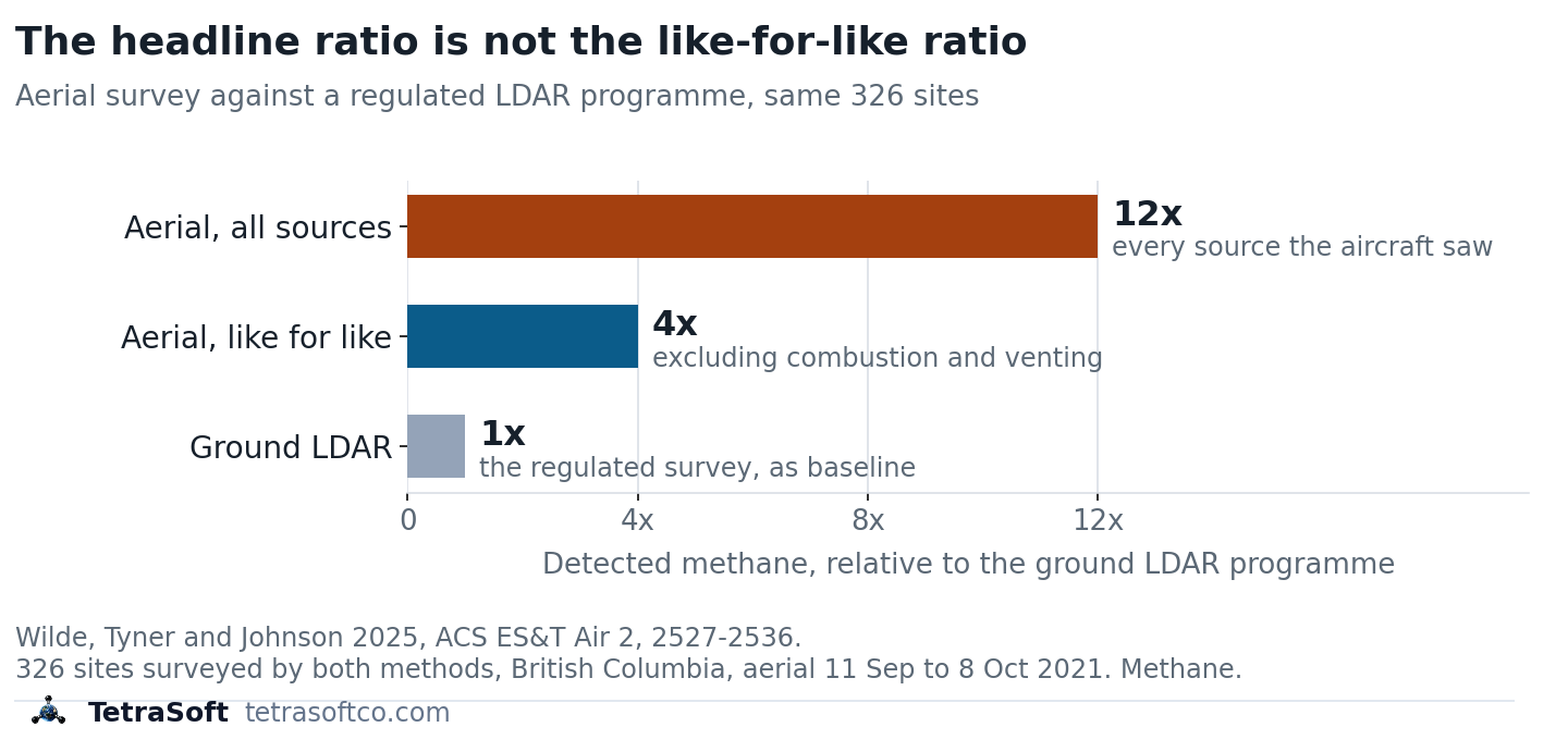
An aircraft study, not a satellite one: the same 326 sites measured two ways, where the like-for-like comparison is fourfold.
The aircraft result matches the satellite pattern: the gap sits in which sources are counted, and how large the rare ones are.
The Leak Detection in Oil and Gas: What Each Method Finds post compares what each measurement method can see.
Why Do Reported and Satellite Methane Differ?
The studies name causes on both sides, and none of them explains the whole gap alone.
What Does the Inventory Miss?
Four gaps show up on the inventory side: rare abnormal events, tanks with failed controls, new wells and flares, and stuck dump valves.
Rare, Large Abnormal Events
Emission distributions “are invariably ‘tail-heavy’, with large emission rates measured at a small subset of sites.” [3] Alvarez and colleagues found the gap is explained if the measurements behind inventory factors “under-sampled abnormal operating conditions.” [3] Shen and colleagues call this a “likely reason” for the gap, pointing to “malfunctions, including fugitive emissions from venting, leakage, inefficient flaring, and blowouts.” [13]
Tanks and Failed Controls
Rutherford and colleagues found tanks and equipment leaks “are the largest contributors to divergence” from the national inventory [14]. The inventory neglects “emissions from failed tank controls (e.g., open thief hatches),” and many of its data sources date from the 1990s [14]. Alvarez and colleagues disagree on that last point, finding outdated component factors “unlikely to explain the difference.” [3]
They differ in method: Alvarez’s team built an EPA-style production inventory from recent component data, and its total came within about 10% of EPA’s [3]. Rutherford’s team used a larger, newer component dataset and added failed tank controls, and its total agreed within error with site-level studies [14].
New Wells and Flares
Citing earlier work, Varon’s team notes “new wells tend to produce high methane emissions in the first few months from well completion and tank flashing.” [9] Satellite plume surveys in the Permian traced 20% of large detections to inefficient flaring [15]. And any facility below the 25,000 ton threshold is absent from the federal inventory but present in the air.
Stuck Dump Valves
Natural gas is mostly methane, with heavier hydrocarbons such as ethane [16]. Separators split the well stream into gas and liquids in stages at falling pressure, and the liquids end in an atmospheric tank [16].
Methane is the most volatile of these hydrocarbons, so at each drop in pressure it leaves the liquid first. Each later stage receives liquid with less methane left in it. The gas that flashes off in the tank is richer in ethane and heavier hydrocarbons, so its ethane-to-methane ratio is higher [16].
When a dump valve sticks open, part of the gas bound for the pipeline passes to the tank and may vent through its relief valve [16]. The site’s vented gas then mixes streams from different stages, so its ethane-to-methane ratio shifts. In Mollel’s simulated facility, the four-hour average ratio moved from about 0.91 in routine operation to 1.69 during the failure [16]. The ratio nearly doubled.
Permian field sampling supports the hypothesis that high-emitting tanks are often caused by “separator malfunctions that leak produced gas through liquids storage tanks.” [17]
What Does the Satellite Miss or Overstate?
Four limits can move a satellite number up or down: detection limits, snapshot timing, model assumptions, and attribution and coverage.
Detection Limits
A point-source imager sees nothing below its threshold, which runs from about 100 to 10,000 kilograms an hour [4]. Smaller sources often go undetected, so a plume survey alone tends to under-count the total even as it catches the large events.
A Snapshot, Not a Year
A satellite pass or a flight captures seconds to a few hours, while an inventory reports a full year [18]. Snapshot methods “provide poor estimates for transient short-duration emitters” and typically fly “during working hours when most maintenance occurs.” [18] Point sources are intermittent: in one survey they produced detectable emissions “only 26 % of the time on average.” [4]
Model Assumptions
Inversion results depend on the prior emissions and background they start from [9]. Lu’s Permian figure “may reflect in part our use of an EPA prior estimate of 0.8 Tg a−1 known to be too low.” [19]
Attribution and Coverage
Inversions often cannot split oil from gas emissions, since “spatial overlap between the two makes specific attribution difficult.” [13] Retrievals need clear skies and work best over bright, uniform surfaces, so coverage is uneven between basins [4].
Get regulatory updates and emissions data insights in your inbox. Subscribe to the TetraSoft newsletter.
How Do You Reconcile a Satellite Number With a Reported Inventory?
One way to reconcile a snapshot with an annual total is to model how often each abnormal event happens and how long it lasts. The tool below converts an observed rate into an annual mass across several durations.
A measurement-informed inventory does that modelling [18]. It uses a mechanistic simulator to combine operators’ inventories with aerial measurements, characterising failure events from site-specific information [18]. OGMP 2.0 Level 5, the top level of the UNEP-hosted methane reporting framework, asks companies to reconcile source-level inventories with site-level measurements [20].
What Do the Appalachian and Denver-Julesburg Studies Show?
In Colorado’s Denver-Julesburg Basin, a study led by TetraSoft cofounder Arthur Santos found 16.4% more emissions than operators reported to the state, from abnormal events [18]. The Colorado surveys, by Carbon Mapper aircraft, had a detection limit of 50 to 150 kilograms an hour [18]. Because of that limit, the authors say the result likely represents a lower bound [18].
A second study Santos led covered 19 midstream sites in the Appalachian Basin [21]. Adding measured abnormal emissions put modelled totals 58.9% above normal-operation GHGRP totals, fugitives excluded [21]. The Appalachian sites were surveyed quarterly by Bridger Photonics’ aerial lidar, which detects much smaller emissions [21]. A Bridger-led assessment across 12 basins put the lidar’s average emission rate detected with 90% probability at 1.27 kilograms an hour in 2023 [22].
The lidar’s lower detection limit may contribute to the larger Appalachian share. The two studies also differ in segment, baseline and state, and differences in state regulation and enforcement may contribute as well.
Where Do MAES and the Reported Numbers Fit?
MAES gives the expected range for a site, and the reported numbers to set beside it are public filings.
MAES, the Mechanistic Air Emissions Simulator, is the model behind both studies [18]. [21] It models normal operation plus common failure modes, such as stuck dump valves, rather than a single average factor [16]. Its Monte Carlo iterations return a range of expected emissions for the site [16].
A satellite or aircraft result can be tested against that range. Pairing that range with field measurements helps an operator pick a survey whose detection limit suits the site [21].
The reported side sits in TetraSoft Atlas, our subscription platform joining public well, production and emissions records. Atlas covers eight states that produced 68 percent of US crude oil and 83 percent of US marketed gas in 2025 [23]. We plan to expand it to every US state [24]. In Colorado it links ONGAEIR facility reports to the wells they list: 38,429 wells whose most recent linked report is for 2025 [25].
This post’s author, Arthur Santos, co-authored the MAES and measurement-informed inventory studies cited here and co-founded TetraSoft. MAES was developed through research that includes the EEMDL initiative of CSU and UT Austin, and TetraSoft offers it through a special license with CSU [26].
Frequently Asked Questions
What happened to the methane satellite?
MethaneSAT, the Environmental Defense Fund’s satellite, lost contact on June 20, 2025 [27]. EDF said the satellite is likely not recoverable [27]. Other methane satellites, including TROPOMI, continue to operate.
Can LiDAR detect methane?
Yes: airborne gas-mapping lidar measures methane along a laser path from an aircraft [28]. One peer-reviewed assessment by Bridger and academic authors put the average rate detected with 90% probability at 1.27 kilograms an hour for 2023 sites [22]. In single-blind controlled-release tests, 87.3% of its emission estimates fell within a factor of two of the true rate [28].
How do I convert CH4 to CO2 equivalent?
Multiply the methane mass by its global warming potential [1]. Over 100 years a tonne of fossil methane is about 30 tonnes CO2e, and over 20 years about 83 [1]. Reports state which horizon and values they use, so check before comparing two CO2e totals.
Have a satellite or aircraft result you need to explain? Contact us to build a measurement-informed inventory for your sites.
This post is for informational purposes only and does not constitute legal or compliance advice. Consult qualified legal counsel or a compliance professional for guidance specific to your operations and jurisdiction.
References
- IPCC AR6 WG1, Chapter 7, Table 7.15. https://www.ipcc.ch/report/ar6/wg1/chapter/chapter-7/
- Zhang et al., 2020, Science Advances, 6, eaaz5120, DOI 10.1126/sciadv.aaz5120. https://doi.org/10.1126/sciadv.aaz5120
- Alvarez et al., 2018, Science, 361, 186-188, DOI 10.1126/science.aar7204. https://doi.org/10.1126/science.aar7204
- Jacob et al., 2022, Atmospheric Chemistry and Physics, 22, 9617-9646, DOI 10.5194/acp-22-9617-2022. https://doi.org/10.5194/acp-22-9617-2022
- EPA, Subpart W revisions, 89 FR 42062, May 14, 2024. https://www.federalregister.gov/documents/2024/05/14/2024-08988/greenhouse-gas-reporting-rule-revisions-and-confidentiality-determinations-for-petroleum-and-natural
- 40 CFR 98.231, reporting threshold for petroleum and natural gas systems. https://www.ecfr.gov/current/title-40/section-98.231
- 90 FR 44591, reconsideration of the Greenhouse Gas Reporting Program, September 16, 2025. https://www.federalregister.gov/documents/2025/09/16/2025-17923/reconsideration-of-the-greenhouse-gas-reporting-program
- 40 CFR 98.238, definitions for petroleum and natural gas systems. https://www.ecfr.gov/current/title-40/section-98.238
- Varon et al., 2023, Atmospheric Chemistry and Physics, 23, 7503-7520, DOI 10.5194/acp-23-7503-2023. https://doi.org/10.5194/acp-23-7503-2023
- Nesser et al., 2024, Atmospheric Chemistry and Physics, 24, 5069-5091, DOI 10.5194/acp-24-5069-2024. https://doi.org/10.5194/acp-24-5069-2024
- Foulds et al., 2022, Atmospheric Chemistry and Physics, 22, 4303-4322, DOI 10.5194/acp-22-4303-2022. https://doi.org/10.5194/acp-22-4303-2022
- Wilde et al., 2025, ACS ES&T Air, 2, 2527-2536, DOI 10.1021/acsestair.5c00195. https://doi.org/10.1021/acsestair.5c00195
- Shen et al., 2022, Atmospheric Chemistry and Physics, 22, 11203-11215, DOI 10.5194/acp-22-11203-2022. https://doi.org/10.5194/acp-22-11203-2022
- Rutherford et al., 2021, Nature Communications, 12, 4715, DOI 10.1038/s41467-021-25017-4. https://doi.org/10.1038/s41467-021-25017-4
- Irakulis-Loitxate et al., 2021, Science Advances, 7, eabf4507, DOI 10.1126/sciadv.abf4507. https://doi.org/10.1126/sciadv.abf4507
- Mollel et al., 2025, ACS ES&T Air, 2, 723-735, DOI 10.1021/acsestair.4c00168. https://doi.org/10.1021/acsestair.4c00168
- Caulton et al., 2023, Elementa, 11, 00121, DOI 10.1525/elementa.2022.00121. https://doi.org/10.1525/elementa.2022.00121
- Santos et al., 2025, ACS ES&T Air, 2, 1598-1611, DOI 10.1021/acsestair.5c00089. https://doi.org/10.1021/acsestair.5c00089
- Lu et al., 2023, PNAS, 120, e2217900120, DOI 10.1073/pnas.2217900120. https://doi.org/10.1073/pnas.2217900120
- OGMP 2.0, Frequently Asked Questions, ogmpartnership.org. https://www.ogmpartnership.org/frequently-asked-questions
- Santos et al., 2026, Gases, 6, 44, DOI 10.3390/gases6030044. https://doi.org/10.3390/gases6030044
- Thorpe et al., 2024, Remote Sensing of Environment, 315, 114435, DOI 10.1016/j.rse.2024.114435. https://doi.org/10.1016/j.rse.2024.114435
- U.S. Energy Information Administration, crude oil and natural gas marketed production by state, annual 2025, accessed September 23, 2026. https://www.eia.gov/dnav/pet/pet_crd_crpdn_adc_mbbl_a.htm and https://www.eia.gov/dnav/ng/ng_prod_sum_a_EPG0_VGM_mmcf_a.htm
- TetraSoft Atlas landing page, tetrasoftco.com/atlas-landing.html, accessed September 30, 2026. https://www.tetrasoftco.com/atlas-landing.html
- TetraSoft Atlas canonical store, counted September 30, 2026. https://www.tetrasoftco.com/atlas-landing.html
- TetraSoft, MAES Platform product page, accessed September 23, 2026. https://www.tetrasoftco.com/maes-platform/maes-landing.html
- Environmental Defense Fund, MethaneSAT Loses Contact with Satellite, July 1, 2025. https://www.edf.org/media/methanesat-loses-contact-satellite
- Bell et al., 2022, Elementa, 10, 00080, DOI 10.1525/elementa.2022.00080. https://doi.org/10.1525/elementa.2022.00080
Reconciler
What an observed plume is worth in a year
A survey reports kilograms per hour. An inventory reports tonnes per year. Converting between them needs a duration nobody measured, so this shows the whole range instead of one number.
Enter an emission rate above zero.
Annualised, that plume is worth
0.88 to 87.60 t CH4/yr
depending only on how much of the year it ran. The duration is the unknown.
If it ran for
| Duty cycle | Annual mass | Share of reported |
|---|---|---|
| 1% of the year | 0.88 t | 0.2% |
| 10% of the year | 8.76 t | 1.8% |
| 50% of the year | 43.80 t | 8.8% |
| Continuous | 87.60 t | 17.5% |
What could have detected it
- Optical gas imaging 0.132 kg/h 90% probability of detection at 7 scfh, high-experience LDAR surveyors only
- Handheld laser 0.6 kg/h 90% probability of detection, all four devices tested below this rate
- Aircraft LiDAR 2.3 kg/h 90% probability of detection at 175 m altitude and 3 m/s wind
- Satellite 33.2 kg/h Smallest emission detected in a single-blind test of nine satellite systems
- Aerial survey used in the DJ basin study 50 kg/h Detection limit that excluded most events below this rate
Nothing in this set would have detected it.
Detection floors: Zimmerle et al. 2020 (OGI, 7 scfh at 90% PoD, experienced surveyors only, converted at the paper's 1 scfh ≈ 18.8 g/h); Day, Levin and Zimmerle 2025 (handheld laser, preliminary); Conrad, Tyner and Johnson 2023 (aircraft LiDAR, 175 m and 3 m/s); Sherwin et al. 2024 (satellite, smallest detected 0.0332 t/h); Santos et al. 2025 (DJ basin survey limit).
A detection limit moves with altitude, wind and surveyor experience. These are the published conditions, not universal constants.
Comments
0Share your thoughts. All comments are moderated before appearing.
No comments yet. Be the first to share your thoughts!